Documentation

Everything you need to get the most out of AriaDNA — a browser-native genomic viewer. No install, no upload: your files are parsed and rendered locally.

1. Open the app at ariadna-bio.com/app and pick a tool from the home screen.
2. Open a file with the Open button in the toolbar, or drag a file onto the drop zone.
3. Explore & export — zoom, search, recolor, annotate, then export a figure or data file.

The workspace & tabs

AriaDNA is multi-document. You can keep several files open at once — a tree, a matrix and a genome — each in its own tab. The global tab bar at the top shows every open document across all tools; click a tab to switch, the × to close it, or + to open another file.

• Open as many documents as you need (up to a sensible limit so memory stays healthy).
• Switching tabs is instant — nothing is re-parsed.
• Your workspace survives a page refresh. It is cleared when you close the app (see Privacy).

Sequence FASTA & GenBank viewer

The sequence viewer opens FASTA (.fasta, .fa, .fna) and GenBank (.gb, .gbk) files and lets you explore a genome from the whole-contig overview down to a single base.

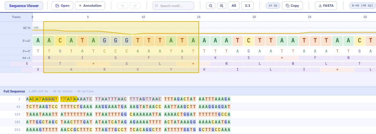
Navigation & reading

• Zoom with the toolbar + / − buttons or the mouse wheel over the canvas. At high zoom you read individual A / T / G / C letters, each color-coded; zoomed out you see the overall base composition.
• Pan by dragging, or use the minimap at the bottom to jump anywhere in the contig.
• Multi-FASTA / multi-contig: if your file has several sequences, switch between them with the contig selector — no need to reload.
• The text panel below the canvas shows the raw sequence; drag its top edge to resize it, or hide it to give the canvas more room.

Features & export

• Annotations: GenBank features (genes, CDS, etc.) are drawn as labeled tracks under the sequence. Hover to see details.
• GC content is plotted as a line so you can spot GC-rich/poor regions at a glance.
• ORFs & translation: open reading frames are highlighted and you can read the live amino-acid translation of a region.
• Search for a motif or subsequence from the toolbar; matches are highlighted on the canvas.
• Export the sequence (or a selection) as FASTA, or features as GFF3, from the side panel.

Alignment Multiple sequence alignment

Open aligned files (.afa, .aln, .msa, or an aligned .fasta) to inspect a multiple sequence alignment.

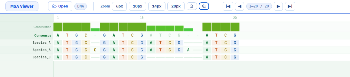
• Colored columns make conserved and variable positions obvious; gaps are shown distinctly.
• The conservation bar under the alignment summarizes agreement per column, and the consensus row shows the dominant residue.
• Zoom from a bird's-eye view of thousands of columns down to single-residue detail; the horizontal scrollbar moves you along the alignment.
• Hover a column to read its position and composition.

Sanger Chromatogram viewer

Open an .ab1 trace to inspect the four-channel Sanger chromatogram, check quality, and correct base calls.

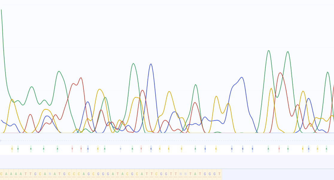
• The four colored traces are the dye channels; the called base sits above each peak, with its quality (QV) reflected in the display.
• Scroll/zoom along the read to inspect noisy regions or low-quality tails.

Editing base calls

You can replace a miscalled nucleotide directly:

1. Click a base on the trace (or its position in the side panel) to select it.
2. Type the correct letter (A, C, G or T). The edit is applied to that position.
3. Repeat for any other positions you want to fix.
4. Export the corrected read as FASTA from the side panel when you're done.

Phylogenetics Tree builder & viewer

The tree tool either loads a Newick tree (.nwk, .tre) or builds one from a distance/profile matrix (.tsv, .csv). It's the richest viewer — here's how to use its main features.

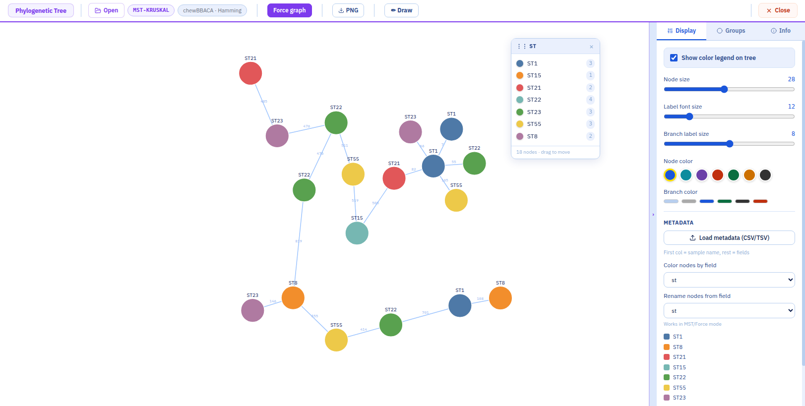
Building a tree

When you open a matrix, AriaDNA asks which algorithm to use. Pick the one that suits your data:

• Neighbor-Joining (NJ) — general-purpose distance tree.
• UPGMA — assumes a molecular clock (ultrametric).
• MST — minimum spanning tree (Kruskal or Prim).
• GoeBURST — for allelic profiles (MLST-style) and clonal complexes.

If you already have a Newick file, just open it and the tree is drawn directly.

Adding metadata

Metadata lets you color and annotate tips by a property (country, year, ST, source…). It's a separate table you load into the open tree:

1. Open the tree's side panel (right edge).
2. Use Upload metadata and choose a .tsv/.csv file. The first column must match the tip/leaf names in the tree; the remaining columns are your metadata fields.
3. Pick the field you want to visualize from the dropdown. Each distinct value gets a color, and a legend appears.

Displaying it differently (layouts)

Switch the tree's shape from the toolbar to suit your story:

• Rectangular — classic dendrogram, best for reading labels.
• Circular — compact for large trees, great for publication figures.
• Force / unrooted — a force-directed network view of relationships.

You can also toggle the legend, adjust tip/label visibility, and highlight a clade.

Drawing & annotating

The draw overlay lets you mark up the tree on top of the canvas — useful for highlighting clusters before exporting a figure.

1. Enable draw mode in the side panel.
2. Choose a shape (e.g. highlight band / blob), a color, and an opacity.
3. Draw over the region or clade you want to emphasize.
4. Combine with metadata colors and the legend, then export your annotated figure.

Matrix Distance & allelic heatmaps

Open a matrix (.tsv, .csv, .tab) to view it three ways, switchable from the toolbar:

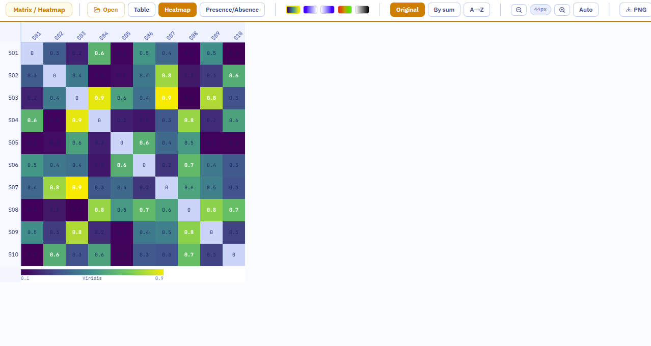
• Table (default) — the raw values, sortable, with a row filter and font-size zoom.
• Heatmap — values mapped to a color scale you can change; zoom adjusts cell size.
• Presence / absence — binary view above a threshold you set.

• Reorder & recolor rows/columns; sort by sum or alphabetically.
• Export PNG of the heatmap or presence/absence view for publications.

Variants · Reads · BLAST

AriaDNA also opens variant and alignment results:

• VCF (.vcf) — browse variants and triage with type and quality filters.
• SAM/BAM (.sam) — inspect read pileups and coverage.
• BLAST (.tsv / .xml / .json) — browse hits sorted by identity and e-value.

Privacy & storage

AriaDNA runs entirely in your browser. Files you open are never uploaded — parsing and rendering happen on your machine.

• Your open documents are saved locally in your browser (IndexedDB), so a refresh keeps your workspace.
• When you close the app, the anonymous workspace is cleared on next launch — nothing lingers.
• Storage is capped and self-managing: the least recently used documents are evicted before it can grow too large.